Author: loganreynolds

For this week’s blog post, I chose to read the short story “That First Time” by Christopher Coake. This story appeared in 2007 in the Granta 97: Best of Young American Novelists 2 and uses third person narration to chronicle Bob “Bobby” Kline’s retrospective discovery after he is notified about the death of a woman whom he briefly hooked up with when he was 17 years old, Annabeth “Annie” Cole, by her best friend, Vicky Jeffords. Nearly 20 years later, Bob is forced to recognize his responsibility in breaking another’s heart, only to learn her best friend had been in love with her the whole time. The narrator illuminates the pain of death with the pain of divorce, using Bobby’s incipient divorce as a vessel for him to understand the depth of the pain of others.

Although there are very few characters in the story (relative to longer, more developed stories), I chose to first create my edge list based on character name and with whom they appeared in a scene or recalled memory with. Bobby Kline transitions between his qualms with the present to his qualms from his past, so I determined this a “scene” when characters were mentioned together. Additionally, I added a third column of weight, which is based on the number of scenes the characters appeared in together—the higher the number of scenes, the higher weight the relationship was given.

I created my network graph via Google Fusion Tables and can be seen below as well as accessed here. I chose to not change the color based on column because my network graph is only between unique characters and no other entities.

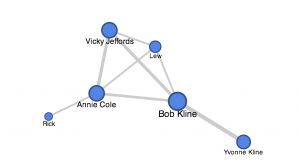
The size of the circle (node) is based on how many unique characters the person appeared in a scene with. For example, Bob, the main character by which the story is centered around, has the largest circle because he appears in a scene with nearly every character. Moreover, the width of the line extending between the nodes is my weight component from the edge list, so a thicker line denotes that the characters appeared in multiple scenes/memories with one another.

On an initial viewing of my network graph, one would be able to discern that Bobby is most likely the main character, due to the size of his node as well as the weights of his edges/lines. The interconnection between Annie, Vicky, Bobby, and Lew brings attention to a possible significant relationship. Yvonne is Bobby’s soon-to-be ex-wife, and my network graph shows how this relationship is significant (by weight) but also isolated from the rest of the characters.

I actually enjoy the shape my network graph took on because the square between Bobby, Annie, Vicky, and Lew almost resembles the table by which they sat at in a pizza restaurant during their adolescence in one of Bobby’s memories. This meeting ultimately transpired into Bobby and Annie’s brief and fleeting relationship that concluded in her heartbreak.

However, my network graph also has significant limitations that ought to be addressed. Although “That First Time” uses third person narration as its mode, the story is told through Bobby’s lens and thus the relationships are within that context. Rick the man who Annie married; however, my network graph shows this relationship as insignificant (if evaluated based on size and appearance). This is because Rick is briefly mentioned in the story, as most of it is recalled from a memory of being 17, which was before Annie met Rick. This limitation occurred based on the ontology I created for my edge list because I used “weight” based simply on how many scenes the characters appeared in together in the story. However, if I used weight based on my understanding of how “strong” the relationship is (i.e. marriage, engagement) then Rick and Annie’s relationship would appear much stronger.

For this week’s mapping exploration, I chose to look at Locating London’s Past, mainly because I do not consider myself well-versed in London’s extensive history and I thought it would be indicative of Turnbull’s arguments to see how this map would be received from someone who has little/no contextual knowledge of the subject.

Locating London’s Past was created by a team of different UK-based universities and offers a virtual exploration of life in “early modern and eighteenth century London” through a variety of different digital databases with records of crime, poor relief, taxation, elections, local administration, plague deaths and archaeological finds sourced from resources from the Old Bailey Online, London Lives, and the Centre for Metropolitan History. In turn, the different data sets are able to be

mapped on three different maps—a GIS compliant version of John Rocque’s 1746 map of London, the first accurate OS map of London (1869-80), and a current Google Maps version.

The project does not claim to offer an exhaustive account of London’s history nor to showcase a particular demographic, but rather leaves data exploration and narrative construction up to the user because truthfully, little guidance is given on what to do. That being said, this mapping project is still largely

an operating example of Turnbull’s contention that all maps are perspectival and subjective because “what is on the map is determined not simply by what is in the environment but also by the human agent(s) that produced it” (Exhibit 2, Page 1). For example, the contributors to Locating London’s Past chose to only include data from legalized sources and the data is limited for it only includes records for crime, taxation, elections, etc. Moreover, the project cites information about each data set on the Historical Background page. For the Old Bailey Proceedings Online data set, the project notes that the original public collections were “inexpensive and targeted initially at a popular audience”, meaning the original versions were designed to sell—not give completely accurate information. Additionally, it cites more “significant limitations” because only half of the editions survived and the recorded transcripts were “selective.” It took a little bit of digging to find this information and it is not openly asserted that the information used for the mapping is largely inconclusive. Nevertheless, the project still chose to use this data for mapping purposes.

This map largely reflects a government’s point of view because the included data has origins from the governing body—using tax, death, crime, and poor relief records as historical indicators. I think it also reflects the point of the view of the group of universities that chose the particular databases as they deemed the particular records as important by choosing them to be a part of the project. A team of different universities might have chosen completely different digital resources to map for a different agenda. The maps operate more as an accessory to the data rather than vice versa because the user must choose a dataset to map rather than to use a map to explore data. Also, not all data records are able to be mapped at all.

This project is able to reveal how certain records are spatially relative to one another and how they could compare in different representations/interpretations of the landscape for a given time period. It obscures how these events are historically relative to one another and contribute to the London’s development. I think “Locating London’s Past” tries to operate on the basis of representing information in an “objective” way to present history (although Turnbull argues this is impossible to do) and thus provides little-to-no narrative on how the maps and datasets relate to one another. As of now, I feel as though I’m just clicking on different data sets and looking at random points. If I were to reimagine a new map, I would provide a narrative on what the map is designed to be used for, and how its presence could be utilized for the understanding of an occurrence without trying to remain neutral because there’s no way to do so anyways.

http://introducingamericanfashion.com/logansfiles/index.html

For this week’s assignment I chose to look at the Economic Dataset from here. The data types consist of the Post-WW2 Election Year and the Unemployment Rate, Inflation Rate, Presidential Approval, and Consumer Confidence for that given year. Original data comes from the Federal Reserve Economic Data (FRED), a Gallup Poll, and a University of Michigan study on consumer confidence. I thought providing a visualization for this set would allow us to get a better understanding of economic trends, how they relate to one another, and provide us with a better direction for further research.

I chose to work with Google Fusion Tables to create a linear graph (“continuous variable chart”) using year on the X-axis and the numerical rating on the Y-axis for both the unemployment and inflation rate. I used this type of visualization so we could better understand how these rates have changed over time as well as how they may relate to one another. The visualization is below and can be accessed here as well.

Unemployment & Inflation Rate by Year

In Data Points, Nathan Yau discusses several visual cues and principles that we are built to recognize and make sense of—I kept these all in mind to create a visualization that would be well-received by the viewer. First, I used the visual cue of position by choosing a continuous variable chart because the viewer will first look to each point and where it is relative to others to understand it. I chose the “continuous” graph instead of a scatter plot so there would be a line created, thus allowing the longer segments in the graph to communicate a significant change. Lastly, the angle and direction of the continuous shape show sharp increases and decreases in the data to allow the viewer to quickly determine differences in the graph so further investigation can be taken.

By using these principles to guide the creation of the data visualization for the Economic Dataset, it’s much more visible and clear that the inflation and unemployment rate tend to change with one another; meaning, unemployment tends to rise as the inflation rate rises. This does not show causation but rather these two economic indicators are most likely affected by the same variables. However, we also notice a breach in this assumption in the years 1948 and 1980. In 1980, inflation shot to a record 14.2, while unemployment was comfortably at 6.3 and descending. This occurrence is able to be clearly seen through my data visualization due to the spatial gap and positioning that communicates an obvious breach/gap from the normal trend. Although this information is present in the original spreadsheet, it was nowhere near as apparent because the spatial gap and change in direction are not visible in the spreadsheet.

After being able to analyze the trends from the data visualization, it would allow me to take a more specific direction if I were to continue economic research. For example, I would obviously look to the economic and fiscal policy that governed the late 1970’s-early 1980’s to try and analyze why/how the inflation rate increased to such a high rate so quickly while the unemployment rate was descending and at a comfortable rate. I could also use this to create a humanities research question, using literature, movies, or songs that discuss the consequences of the high inflation rate as an indicator for the social sentiment of the time period. Whichever research direction I decided to take, whether it be policy or humanities driven, the decision can be attributed to the findings from my data visualization that showed me variables that are worth further investigation. I also acknowledge that much more advanced data visualizations could be constructed from this data but as a beginner I thought this was a simple visualization that had great impact!

Before diving into the creation of my own blog post for this week, I examined the ones already posted by classmates to read about the different datasets they chose from the L.A. Controller’s Office platform. I enjoyed this one especially because it used the concept of digital division discussed by Wallack and Srinivasan as a lens to evaluate the platform itself by noting how the popularity/value of each set (measured by # of views) could be an implication of the “mismatched ontologies between the state and individuals.”

Taking this notion into account, I used the drop down menu on the left to view the popularity of the different sets this past week, month, and year. As the police force continues to be a large part of national discussion, I decided to choose the Police Expenditures dataset. I think it is particularly reflective of public sentiment (and thus possibly community ontology) that this dataset was one of the most viewed for the year (although not for this week or month).

As denoted by the title, this dataset contains information regarding the police force’s expenditures from June 2011-January 2014. There are 25 data types consisting of ID Number, Fiscal Year, Department Name, Vendor Name, Transaction Date, Dollar Amount, Authority, Business Tax Registration Certificate, Government Activity, Fund Group Name, Fund Type, Fund Name, Account Name, Transaction ID, Expenditure Type, Settlement/Judgment, Fiscal Month Number, Fiscal Year-Month, Quarter, Calendar Month #, Calendar Month Year, Calendar Month, Data Source, Authority Name, and Authority Link. A record for this dataset is a single purchase (expenditure) made by a department within the L.A. Police Force.

Wallack and Srinivasan first discuss the importance of ontology by stating, “Ontologies represent reality, but this representation of information may in turn become the basis for actions that in turn shape reality” (3). They then proceed to delineate the differences between meta ontologies and localized, community ontologies and the consequences when there are discrepancies between the two. Based on their definitions, I would say the Police Force Expenditures dataset is a meta ontology based on the criteria of its data types. For example, ID Number, Business Tax Registration Certificate, Fund Group Name, Fund Type, and Transaction ID are all types that make little to no sense to local citizens. These types are only understood by government and city officials that work with and understand the particular taxing and funding protocol. Although it should be noted that other data types are able to be understood by non-government workers such as the Dollar Amount and Vendor Name.

This dataset can tell you about the money that was spent by a police department, for each record indicates a specific expenditure made by a department with a dollar amount and to which vendor it was paid for. However, the item or service that was purchased is not specified, only the “Government Activity” it was used for, which is rather broad considering nearly all of records have “Protection of Persons and Property” as the reason for activity. Thus, I think this dataset is only informative for quantifying purchases for the different departments, rather than trying to determine exactly what each spends their money on specifically.

If I were to create a local, community ontology on Police Expenditures the data types would not look entirely different, rather I would take away and add a few data types. I think the general public would primarily want to know an itemized list of the specific goods and services purchased by the department from the vendor and a more informative reason as to why such purchase was made. I would still collect the same data regarding the dollar amount, vendor name, department, and fiscal time periods; tax registration and identification numbers are not essential for the community ontology.

In his examination of the intersection between “event” and “history” in his essay “The Value of Narrativity in the Representation of Reality,” Hayden White argues that the moral presence concerning the way in which the world operates ultimately forms the narrative to write history. To formulate such notion, White states, “historical self-consciousness, the kind of consciousness capable of imagining the need to represent reality as a history, is conceivable only in terms of its interest in law, legality, legitimacy, and so on” (17). In essence, our idea of history is constructed by a slew of events. We relate these events through a cause-and-effect relationship that we base on our idea of how the world works.

Taking this notion into account, we can use this idea of narrative forming history in the context of archives. Specifically, I chose to examine the Collection of Material about Japanese American Internment, 1929-1956 because as someone with Japanese ancestry, I felt that this archive is the one that resonates most with me. I also thought the narrative that I would construct from the material would possibly be different from someone who does not have a similar background, thus showcasing the implications of White’s original argument.

The collection consists of materials from the War Relocation Authority (WRA) under the U.S. Department of the Interior. Materials include pamphlets, press releases, yearbooks, speeches, theses, and more writings regarding the conditions in the camps, detailing of the internment process, Japanese relocation after war, and more. The first two boxes containing the WRA material are organized chronologically and thus eases the process in formulating a narrative because it can follow a trajectory based on a timeline. I would begin in the Spring of 1942, detailing the initial conditions of internment and Japanese relocation, signifying World War II as the cause of such occurrences. Initially, conditions seem are relatively unknown but progressively show to only grow worse, denoted by the “Tule Lake incident” and “demonstration at Tule Lake Hospital” of the Semi-Annual report of 1943. It only continues to worsen as Tule Lake is shut down entirely in 1946. Moreover, addresses from army officials calling for the “humane treatment of Japanese Americans” demonstrate how the conditions of inhabitants of the camps had grown to inhumane in their execution. Pamphlets detailing anti-Japanese sentiment show the ways in which this treatment was able to persist because of how citizens were taught to view such people.

Other narratives are able to be constructed from the materials in this collection as well, such as ones construed from the yearbooks of the Manzanar camps. Historical narratives regarding the people who inhabited such camps and their daily routines could be constructed from the names and subsequent accounts.

Moreover, I think the larger narratives that can be constructed from the materials could be surrounding the story of Japanese-American life post-WWII. Much of the material is focused on life within the camps and the lives of those who inhabited them. Ironically, this narrative is generally muted in typical conversations of today. This material has the ability to explain part of the silenced story. I do not think this collection has the ability to explain everything from my constructed narrative, however, because much of the material is from WRA (a government agency) and thus most likely does not showcase the true horrendous conditions that Japanese-Americans had to go through. I might remedy this by looking to the first-person accounts as well as other signifiers such as the call for “humane treatment” by Sergeant Ben Kuroki that demonstrate the horrible events that were occurring during this time period. I would potentially fill the gaps within the narrative by stories passed down from my ancestors; however, it should be noted that even most of these stories have failed to continue existing due to their silencing from government urge.