Creating a Network Graph with Gephi
Gephi is a powerful tool for network analysis, but it can be intimidating. It has a lot of tools for statistical analysis of network data — most of which you won’t be using at this stage of your work.
Open Gephi

Be sure you’re on the Windows side of your computer and that you’re opening Gephi version 8.2. (Gephi 8.2 for Mac doesn’t work; if you want to use Gephi at home and you have a Mac, be sure and download 8.1.)
Create a new project

Click on New Project on the “Welcome to Gephi” popup window.
Do not freak out.
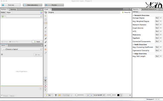
The Gephi workspace looks really confusing and intimidating. Do not freak out.
Click on “Data Laboratory.”
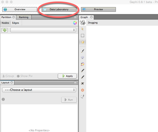
This is where you’ll upload your data.
In the Data Laboratory, click on “Import Spreadsheet.”

Click on Import Spreadsheet in order to upload your data.
Import “dh101nodelist.csv” as a Node table

1) Click on the button with the three dots on it to select a file and click on dh101nodelist.csv.
2) Be sure you choose Nodes table from the box that allows you to choose between an edge table and a node table.
3) Finally, click Next to move on to the next screen, leave the options as they are, and click Finish on the window that follows.
Import “dh101questions.csv” as an Edges table

We’ve told Gephi what the individual nodes are going to be. Now we need to tell it how the nodes are related to each other with an edge table.
1) Click on Import Spreadsheet again.
2) Click on the button with the three dots on it to select a file and click on DH101 6B Dataset 2.
3) Be sure you choose Edges table from the box that allows you to choose between an edge table and a node table.
4) Finally, click Next to move on to the next screen and then Finish on the following screen.
What is this, it’s confusing and I hate it.

The window you see in front of you is Gephi’s Data Laboratory, where you can manipulate the data you’ve uploaded. If you click on the Nodes or Edges tab, you can toggle between the two spreadsheets you uploaded. For the time being, however, we’re not going to change anything.
Click on “Overview.”

OK, we can finally start visualizing. Click on Overview to go to the pane that will show your network graph.
Cool, I guess?

You now have a network diagram! You can’t really see much, though.
Manipulate your diagram so it’s more legible.
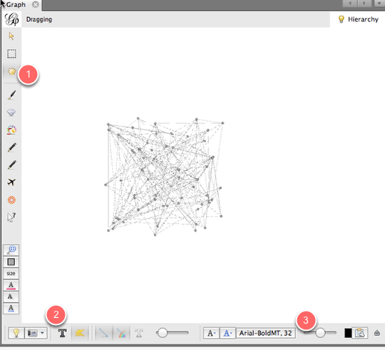
Use the scroll wheel to zoom in and out. 1) Use the hand icon to move the diagram around. (If you’re on a Mac, you’ll need to hold down the command key while you use the little hand.) 2) Turn labels on by clicking the T. 3) Adjust the size of the labels with the scrubber.
What are we looking at?

This is a bimodal network graph, meaning it contains two different kinds of things: students and preferences. Each student is connected to his or her preferences with an edge. It’s still a little hard to see anything, though.
Separate “students” from “preferences.”

Let’s make the student nodes one color and the preferences node another color, so that we can distinguish between students and their preferences. Remember that our node list (dh101nodelist.csv) contained a column called node-type that identified each node as either a student or a preference. We can use that to partition our nodes into two colors.
On the upper left-hand portion of the screen, you’ll see a box that has two tabs: Partition and Ranking. Be sure that the Partition tab is selected (1). (We use the partition tab for this because we’re dividing our nodes into groups. If we were trying to rank our nodes by some value, we’d use the ranking tab.)
Then, within the Partition tab, be sure that the Nodes tab is selected (2). Click the button with the two green arrows to refresh your selection (3). (I don’t know why you have to do this; you just do.) Then, from the dropdown menu, select node-type (4). Finally, click Apply (5).
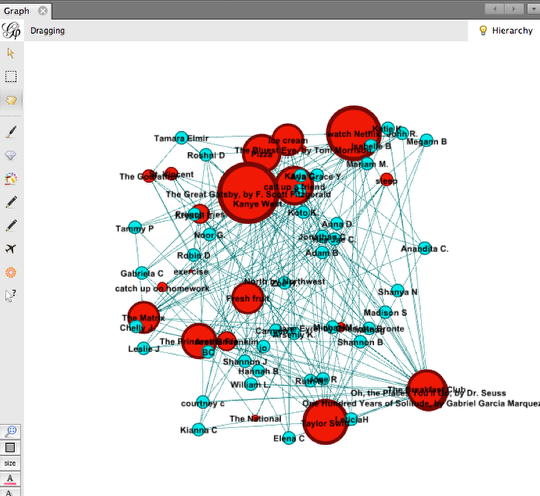
Now you can distinguish students from their preferences.

In my diagram, students are turquoise and preferences are pink.
Calculate average degree.

Let’s make the more popular nodes bigger, to indicate that more students have chosen them.
To do that, we need to calculate the nodes’ Average Degree, meaning the number of inboud and outbound connections to them. To do this, head to the right side of your Gephi window, where you’ll find a Statistics page. Click the Run button that appears to the right of Average Degree. Then close the Degree report that pops up.
Size nodes according to their popularity.
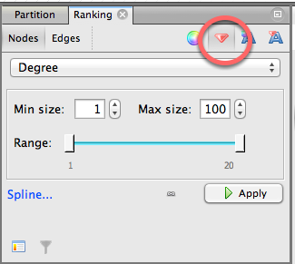
Now let’s use the average degree, which we just calculated, to size the nodes. Head back to the left side of the Gephi window, and this time click on the Ranking tab, because this time we’re not just dividing our nodes into groups; we’re ranking them by average degree.
Within the Ranking tab, click on Nodes, and from the drop-down menu, click on Degree. You can rank nodes in a few different ways, including by color. But let’s use size, which is indicated by the tiny red diamond. Click on the tiny red diamond to rank nodes by size. Then hit Apply.
Now you can see who chose what, and how popular those choices were!